Efficient Graph Storage for Entity Resolution Using Clique-Based Compression

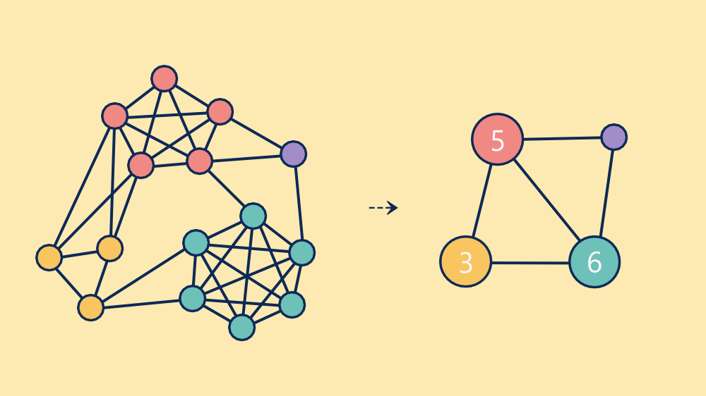
TL;DR: TL;DR Dense entity graphs grow quadratically in edge count as records accumulate, making naive storage unsustainable. Clique-Based Graph Compression (CBGC) solves this by replacing large sets of pairwise edges with compact clique records. In one production deployment, CBGC cut edge storage by 99.7% while preserving full traceability and improving deletion performance.
| Aspect | Naive edge list | With CBGC |
|---|---|---|
| Edge growth formula | n*(n-1)/2 per clique | 1 clique record per complete subgraph |
| Edges for n=1,000 | Up to 499,500 | 1 clique record (+ sparse remainder) |
| Real-world saving | Baseline | 99.7% fewer stored edges (one customer) |
| Traceability | Full (rule ID per edge) | Full (rule ID per clique) |
| Deletion performance | Traverse every edge | Treat clique as pre-connected subgraph |
| Detection cost | N/A | NP-hard (max clique); greedy heuristics in practice |
| Loss-free? | Yes | Yes (unless per-edge properties required) |
On this page
- The Entity Graph Model
- The Scaling Problem: Quadratic Growth
- Solution: Clique-Based Graph Compression (CBGC)
- Performance Benefits Beyond Storage
- Trade-Offs: Clique Detection Complexity
- Beyond Cliques
- Closing Thoughts
- FAQ: Frequently Asked Questions
In the world of entity resolution (ER), one of the central challenges is managing and maintaining the complex relationships between records. At its core, Tilores models entities as graphs: each node represents a record, and edges represent rule-based matches between those records. This approach gives us flexibility, traceability, and a high level of accuracy, but it also comes with significant storage and computational challenges, especially at scale. This article explains the details about efficiently storing highly connected graphs using clique-based graph compression.
The Entity Graph Model
In Tilores, a valid entity is a graph where every record is connected to at least one other via a matching rule. For instance, if record a matches record b according to rule R1, we store that as an edge "a:b:R1". If another rule, say R2, also connects a and b, we store an additional edge "a:b:R2". These edges are kept as a simple list, but could alternatively be modeled using an adjacency list structure for more efficient storage.
Why Retain All Edges?
Most entity resolution systems or master data management systems don’t retain the relationships between records, but only store a representation of the underlying data and typically a generic matching score, leaving the user uncertain about how the entity was formed. Even worse, the user has no way to correct errors made by the automatic matching system.
Hence, retaining all edges in an entity graph serves multiple purposes:
- Traceability: Allows the user to understand why two records were grouped into the same entity.
- Analytics: Insights such as rule effectiveness and data similarity can be extracted from edge metadata.
- Data Deletion & Recalculation: When a record is deleted or a rule is modified, the graph must be recalculated. Edge information is essential to understand how an entity was formed and how it should be updated.
The Scaling Problem: Quadratic Growth
When discussing potential scaling issues in entity resolution, this typically refers to the challenge of matching each record with all other records. While this is a challenge on its own, retaining all edges of an entity results in similar issues on the storage side. Entities where many records are connected with each other create a multitude of edges. In the worst case every new record is connected to all existing records. This quadratic growth can be expressed with the formula:
n * (n - 1) / 2
For small entities, this is not an issue. For example, an entity with 3 records can have a maximum of 3 edges. For n = 100, this increases to 4,950 edges and for n = 1,000 this results in up to 499,500 edges.
This creates an immense storage and computational overhead, especially since entity resolution graphs often exhibit this kind of dense connectivity.
Understanding the scaling challenge is foundational to what entity resolution actually involves at enterprise scale: the matching logic and the graph storage problem are intertwined.
New posts on entity resolution, identity data and AI. No spam, unsubscribe any time.
What Makes Naive Edge Storage Unsustainable at Scale?
For small entities, linear edge lists are manageable. For n=100 records you get 4,950 edges; for n=1,000 you get up to 499,500. Any storage system treating each edge as an independent row pays that cost in full, with no benefit from the structural redundancy that dense cliques represent. The root cause is that naive storage ignores the complete-subgraph structure already present in the data.
Solution: Clique-Based Graph Compression (CBGC)
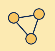
A clique in a graph is a group of nodes where every node is connected to every other node in that group. A clique can also be called a complete subgraph. The smallest possible clique contains a single node and no edges. A pair of nodes connected by an edge also forms a clique. And three nodes, such as the one below, form a triangle shaped clique.
A maximal clique is a clique that cannot be extended by adding any adjacent node, and a maximum clique is the clique with the largest number of nodes in the whole graph. For the purpose of this article, we’re going to use the term clique only to refer to cliques with at least three nodes.
The previously shown triangle could be represented in Tilores by the following edges:
[
  "a:b:R1",
  "a:c:R1",
  "b:c:R1"
]
Because a triangle is a clique, we could also represent the graph by storing only the nodes in this clique and the associated rule ID:
{
  "R1": [
    ["a", "b", "c"]
  ]
}
Let’s consider the following slightly more complicated graph:
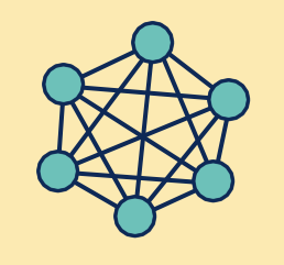
Based on its appearance, we can easily spot that all nodes are connected to each other. So instead of listing all 15 edges [remember n*(n-1)/2], we can simply store this clique in the following form:
{
  "R1":[
    ["a", "b", "c", "d", "e", "f"]
  ]
}
However, in a realistic graph, not all records are connected to each other. Consider the following graph:
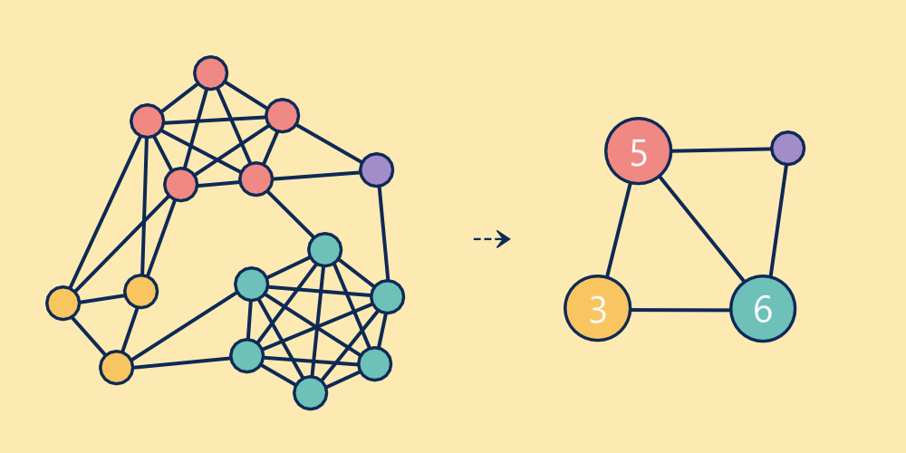
There are three larger cliques highlighted: yellow, red and blue (teal if you’re picky). There is also a single remaining node. While those are probably the largest cliques, you might spot dozens of others. For example, do you notice the 4-node clique between the two red and two yellow nodes?
Sticking with the colored cliques, we could store them in the following way (using y, r and b for yellow, red and blue):
{
  "R1": [
    ["y1", "y2", "y3"],
    ["r1", "r2", "r3", "r4", "r5"],
    ["b1", "b2", "b3", "b4", "b5", "b6"]
  ]
}
Additionally, we can store the remaining 10 edges (p for purple):
[
  "y1:r1:R1",
  "y1:r2:R1",
  "y2:r1:R1",
  "y2:r2:R1",
  "r4:p1:R1",
  "r5:p1:R1",
  "r5:b1:R1",
  "b2:p1:R1",
  "y3:b5:R1",
  "y3:b6:R1"
]
This means that the whole graph can now be represented with only three cliques and ten edges, instead of the original 38 edges.
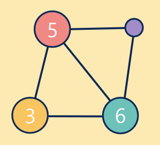
This clique-based graph compression (CBGC) is loss-free (unless you need edge properties). In a realistic dataset, we identified massive storage savings. For one customer, CBGC reduced edge storage by 99.7%, replacing hundreds of thousands of edges with just a few hundred cliques and sparse edges.
This same graph-based approach underpins how entity resolution integrates with master data management, where traceable, correctable entity graphs are a core requirement.
Performance Benefits Beyond Storage
CBGC is not just about compression. It also enables faster operations, particularly when handling record and edge deletion.
Any sane entity resolution engine should split an entity into multiple ones if the only link between two subgraphs was deleted, for example, due to regulatory or compliance reasons. Identifying separate, unconnected subgraphs is typically done using a connected components algorithm. In short, it works by grouping all nodes that are connected via edges into separate subgraphs. As a result each edge needs to be checked at least once.
However, if a graph is stored as a compressed graph, then there is no need to traverse all edges of a clique. Instead it is sufficient to add a limited number of edges for each clique, for example a transitive path between the nodes of a clique, treating each clique as a pre-connected subgraph.
Trade-Offs: Clique Detection Complexity
There is a trade-off: clique detection is computationally expensive, particularly when attempting to find the maximum cliques, a well-known NP-hard problem.
In practice it is often sufficient to simplify this workload. Approximate algorithms for clique detection (e.g. greedy heuristics) perform well enough for most uses. Additionally, CBGC is recalculated selectively, usually when an entity’s edge count surpasses a threshold. This hybrid approach balances compression efficiency with acceptable processing cost.
Research on listing all maximal cliques in sparse graphs in near-optimal time (Eppstein, Loffler and Strash, 2010) confirms that exhaustive enumeration of maximal cliques is tractable for sparse graphs, while dense graphs require the kind of selective, threshold-triggered approach that CBGC applies.
Beyond Cliques
Arguably, the most common pattern in entity resolution is the complete subgraph. However, further optimization could be achieved by identifying other recurring patterns such as
- stars: store as a list of nodes where the first entry represents the central node
- paths: store as an ordered list of nodes
- communities: store like a clique and mark the missing edges
Closing Thoughts
Entity resolution systems often face the challenge of managing dense, highly interconnected graphs. Storing all edges naively quickly becomes unsustainable. CBGC provides an efficient way to model entities by exploiting structural properties of the data.
Not only does it reduce storage overhead, but it also improves system performance, especially during data deletion and reprocessing. While clique detection has its computational costs, careful engineering choices allow us to reap the benefits without sacrificing scalability.
For teams evaluating how to build or integrate an entity resolution system, the tradeoffs around precision and recall in entity resolution sit alongside storage architecture as two of the key engineering decisions.
When Should You Apply CBGC to Your Entity Graph?
CBGC is most valuable when entities with high record counts appear frequently in your dataset. If your graph is sparse and entities rarely exceed a dozen records, the overhead of clique detection may not justify the storage saving. Tilores applies CBGC selectively, triggering recalculation only when an entity’s edge count crosses a threshold, so the technique activates precisely where it delivers the greatest benefit.
See what resolved entity data does for your business — and your AI.
See it on your own data: book a demo for a walkthrough on your records, or get the evaluation build to try resolved entity data locally.
FAQ
What is Clique-Based Graph Compression (CBGC) in entity resolution?
CBGC is a storage technique that replaces dense lists of pairwise edges in entity graphs with compact clique representations. A clique is a group of nodes where every node is connected to every other node. Instead of storing n*(n-1)/2 edges for a fully connected subgraph, only the set of node IDs and the rule ID are stored. This is loss-free unless edge-level properties are required.
Why does edge storage grow quadratically in entity resolution?
In an entity graph, every matching rule between two records creates an edge. When many records in an entity are all connected to each other, the number of edges grows as n*(n-1)/2 (where n is the number of records). For n=100 that is 4,950 edges; for n=1,000 that is up to 499,500 edges. This quadratic growth creates immense storage and computational overhead at scale.
How much storage does CBGC save in practice?
In a real customer deployment, CBGC reduced edge storage by 99.7%, replacing hundreds of thousands of edges with just a few hundred cliques and sparse edges.
Does CBGC improve performance beyond storage savings?
Yes. CBGC also speeds up operations such as record and edge deletion. When running a connected-components algorithm to detect unconnected subgraphs after a deletion, a compressed graph does not require traversing every edge inside a clique. Instead, a limited transitive path per clique is sufficient, treating each clique as a pre-connected subgraph.
What is the computational cost of clique detection?
Finding maximum cliques is an NP-hard problem. In practice, approximate algorithms such as greedy heuristics perform well enough for most entity resolution workloads. CBGC is also recalculated selectively, typically only when an entity’s edge count surpasses a threshold, which keeps the processing cost acceptable.
See what resolved entity data does for your business — and your AI.